Tutorial 1: Theta Phase Precession Analysis

This tutorial walks you through a complete neuroscience analysis workflow in SynapChart — from a raw recording to batch processing across multiple sessions.

By the end you will have:

• Loaded and run a template theta phase precession workflow
• Created a custom block that computes a quantitative metric
• Packaged the entire workflow as a reusable composite block
• Applied that composite block to two recording sessions in parallel

Estimated time: 30–45 minutes
Data: Three synthetic hippocampal recording sessions included in the repository (backend/scripts/)

Before you begin

Make sure SynapChart is installed and running. If not, follow the Getting Started guide first — it covers installation and a full tour of the interface.

---

Part 1 — Get the Test Data

The repository includes three synthetic hippocampal recording sessions in the backend/scripts/ folder. Each session contains three files:

File	Contents
phase_precession_N_lfp.npy	Multi-channel LFP recording (1250 Hz)
phase_precession_N_spikes.npy	Spike timestamps for one place cell (seconds)
phase_precession_N_position.npy	Animal position: columns are time, x, y (30 Hz)

where N is 1, 2, or 3. You can use any session for Parts 1–3.

If you cloned the repository these files are already present. If you installed via pip and want to generate your own copy, run:

python backend/scripts/generate_phase_precession_data.py

---

Part 2 — Run the Template Workflow

2.1 Load the template

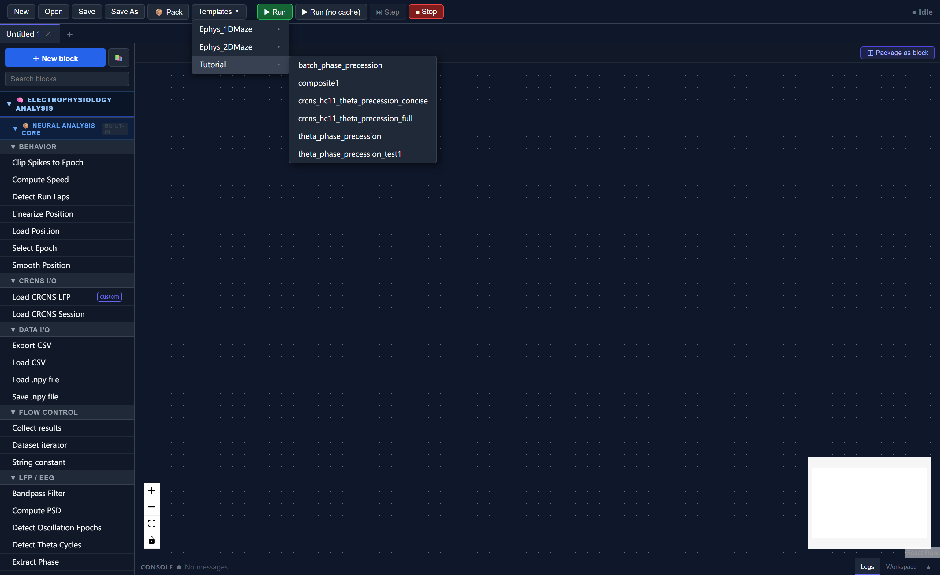
In the toolbar click Templates, expand the Tutorial category, and select theta_phase_precession.

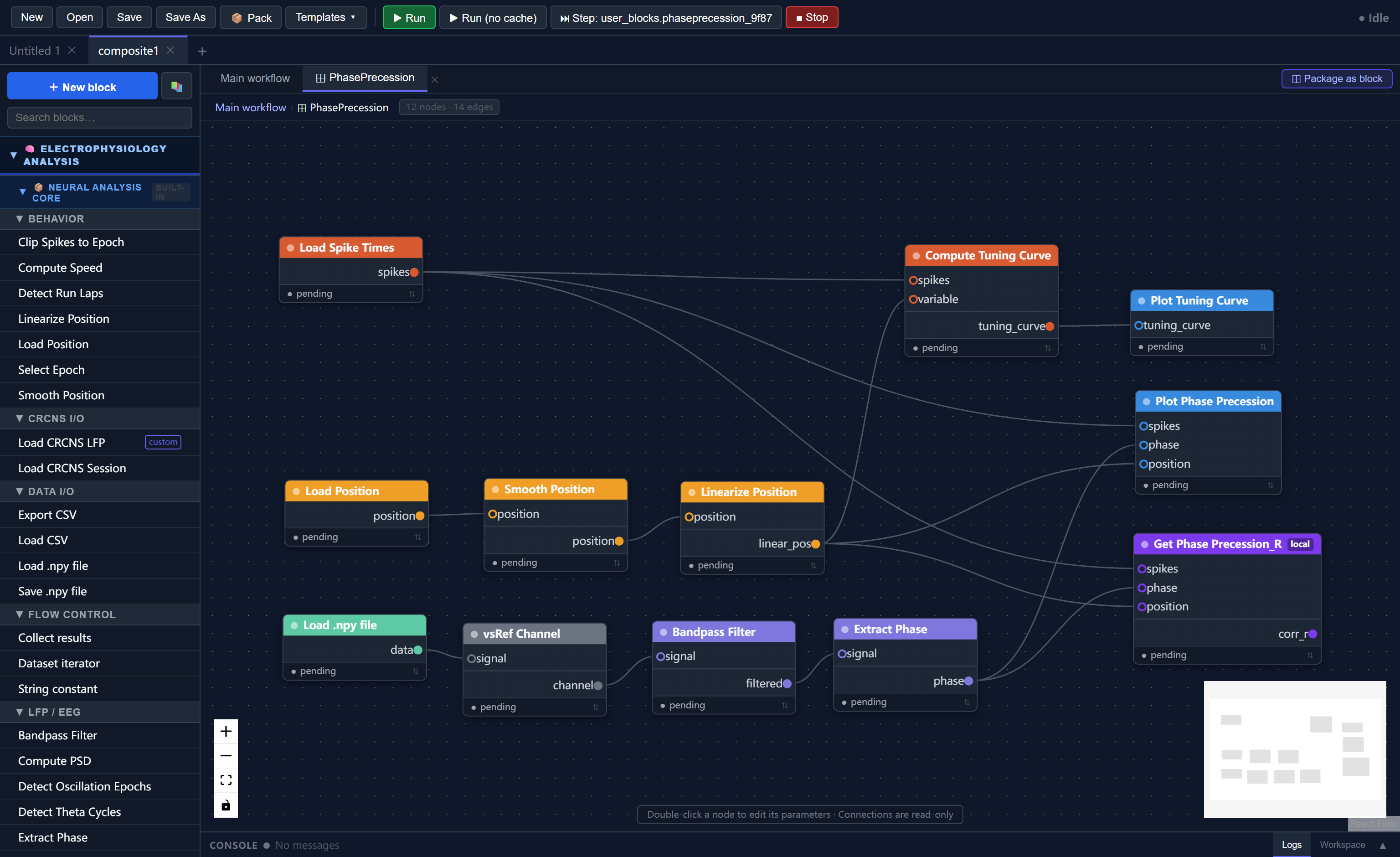
The canvas loads a pre-built pipeline with 10 connected blocks:

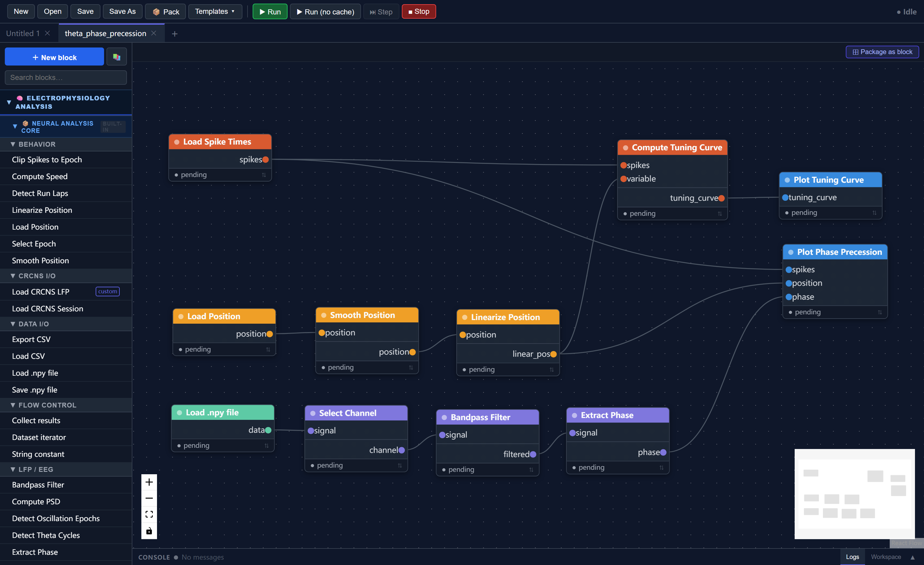
The workflow implements this analysis chain:

Load LFP ──► Select channel ──► Bandpass (4–12 Hz) ──► Extract phase
                                                              │
Load spikes ──────────────────────────────────────────► Phase precession plot
                  │                                           │
                  └──► Compute tuning curve ──► Tuning curve plot
                              ▲
Load position ──► Smooth ──► Linearize

What each stage does:

• Load LFP / spikes / position — reads the three .npy data files from disk
• Bandpass filter (4–12 Hz) — isolates the theta oscillation from the raw LFP
• Extract phase — computes instantaneous theta phase via the Hilbert transform
• Smooth & linearize position — smooths the raw position trace and projects 2D coordinates onto the 1D track axis
• Compute tuning curve — calculates firing rate as a function of position (the place field)
• Plot tuning curve — displays the place field
• Plot phase precession — scatter plot of spike phase vs. position, showing that spikes systematically shift earlier in the theta cycle as the animal crosses the place field

2.2 Set the file paths

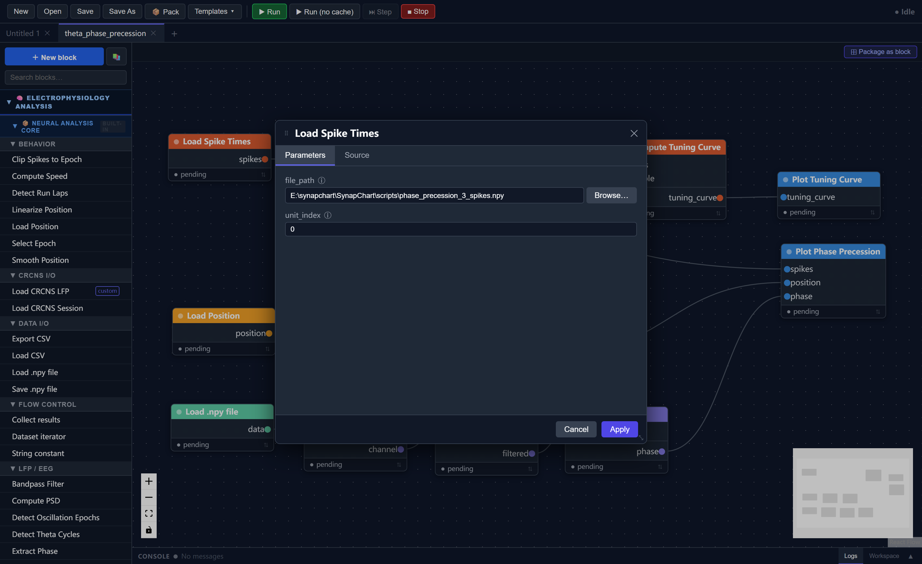
Three blocks need file paths pointing to your data. Double-click each one to open its parameter editor:

Block	Parameter	Value
Load LFP	file_path	path to phase_precession_N_lfp.npy
Load spike times	file_path	path to phase_precession_N_spikes.npy
Load position	file_path	path to phase_precession_N_position.npy

2.3 Run the pipeline

Click Run in the toolbar. The run progress panel expands at the bottom and shows each block executing in order.

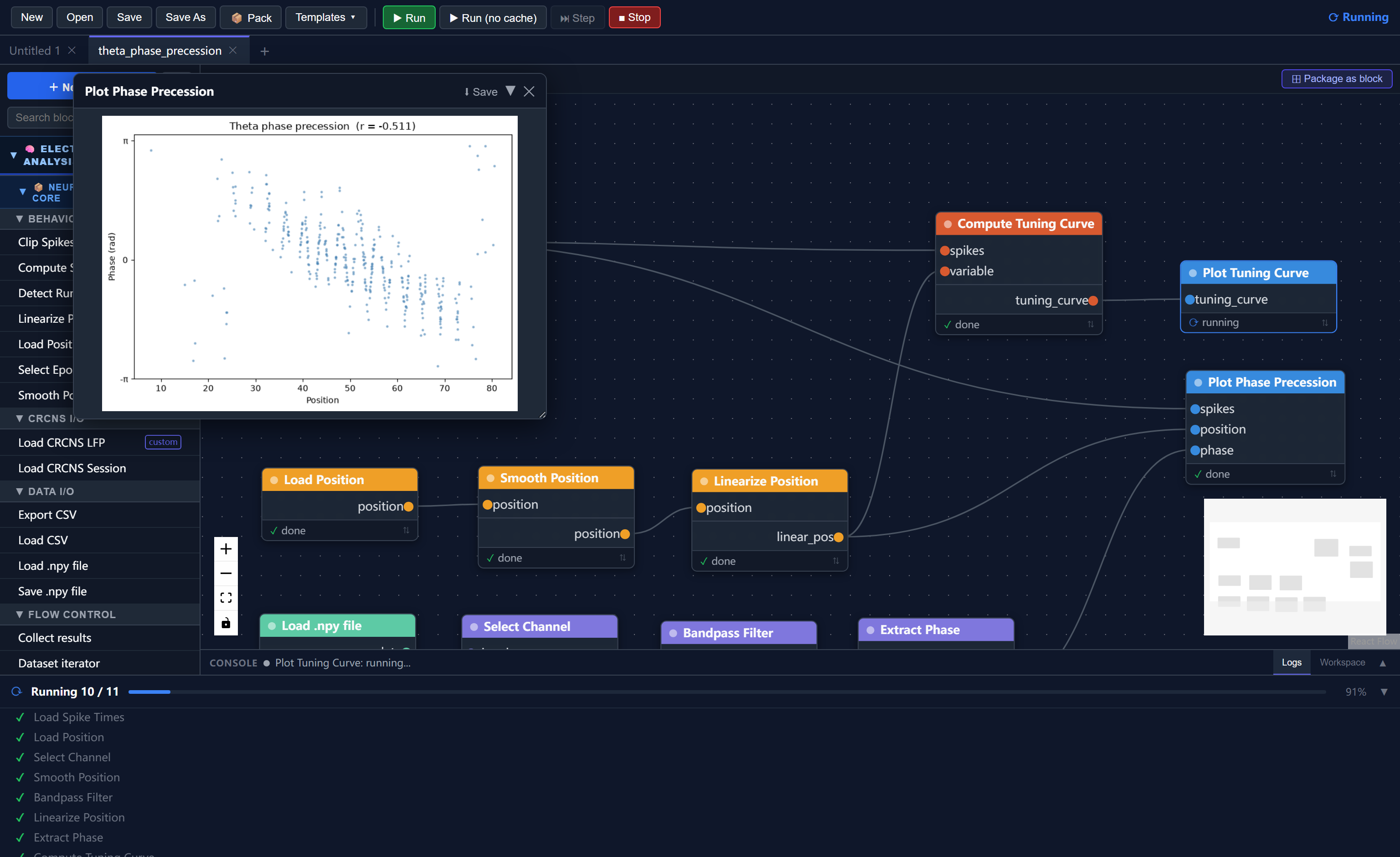
When complete, two visualization windows appear:

• Place field — firing rate as a function of position along the track
• Theta phase precession — each dot is one spike; the downward slope shows that spikes shift to earlier theta phases as the animal moves through the place field

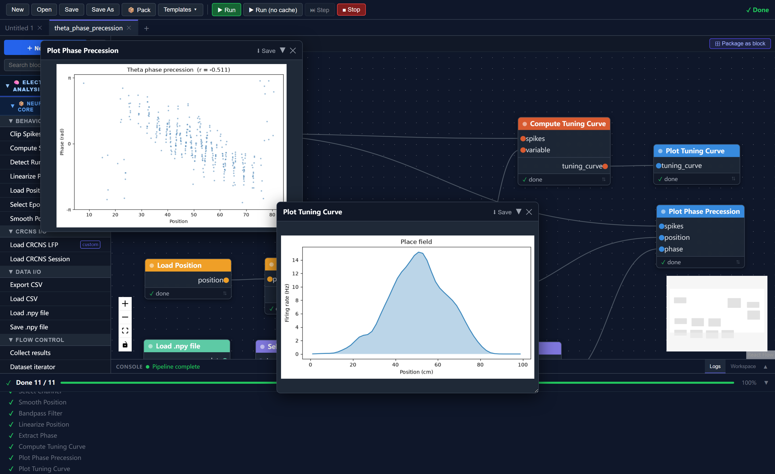
Tip

On subsequent runs, unchanged blocks load from cache automatically — only modified branches re-execute. Change a parameter and only the downstream blocks re-run.

---

Part 3 — Creating a Custom Block

The template visualises phase precession qualitatively. Here you will create a block that quantifies it: computing the Pearson correlation coefficient between spike phase and position. A more negative value indicates stronger phase precession.

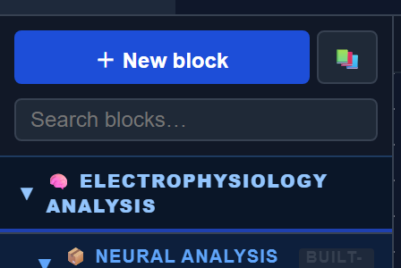
3.1 Open the block wizard

Click + New Block at the top of the side panel.

3.2 Step 1 — Metadata

Field	Value
Block name	Get Phase Precession R
block_type_id	get_phase_precession_r (auto-filled)
Category	Visualization
Description	Computes Pearson correlation between spike phase and position as a measure of phase precession strength.

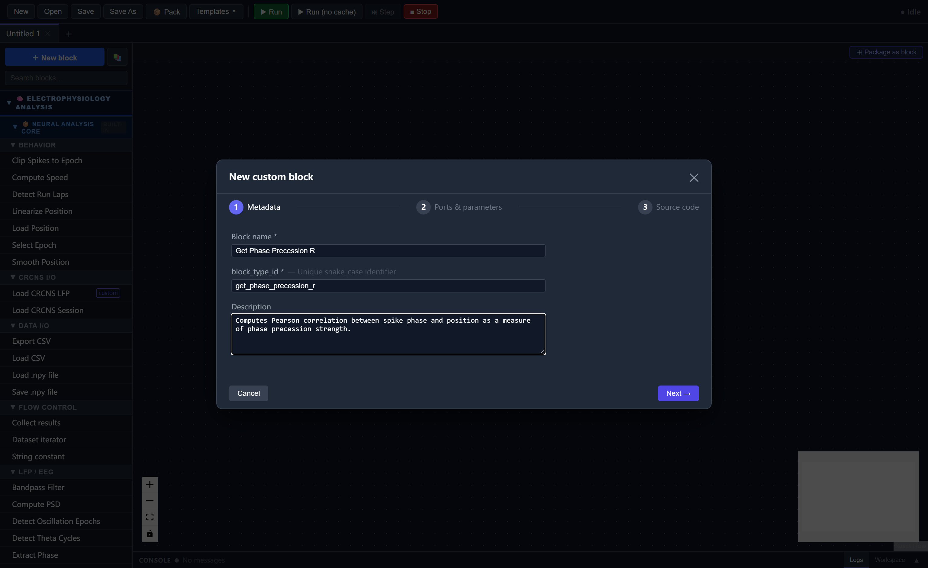
Click Next.

3.3 Step 2 — Ports & Parameters

Inputs — add three rows:

Port name	Data type	Description
spikes	NeuroData[spike_times]	Spike timestamps
phase	NeuroData[raw_signal]	Instantaneous LFP phase
position	NeuroData[position]	Linearized position

Outputs — add one row:

Port name	Data type	Description
corr_r	float	Pearson r (phase vs. position)

Parameters — leave empty.

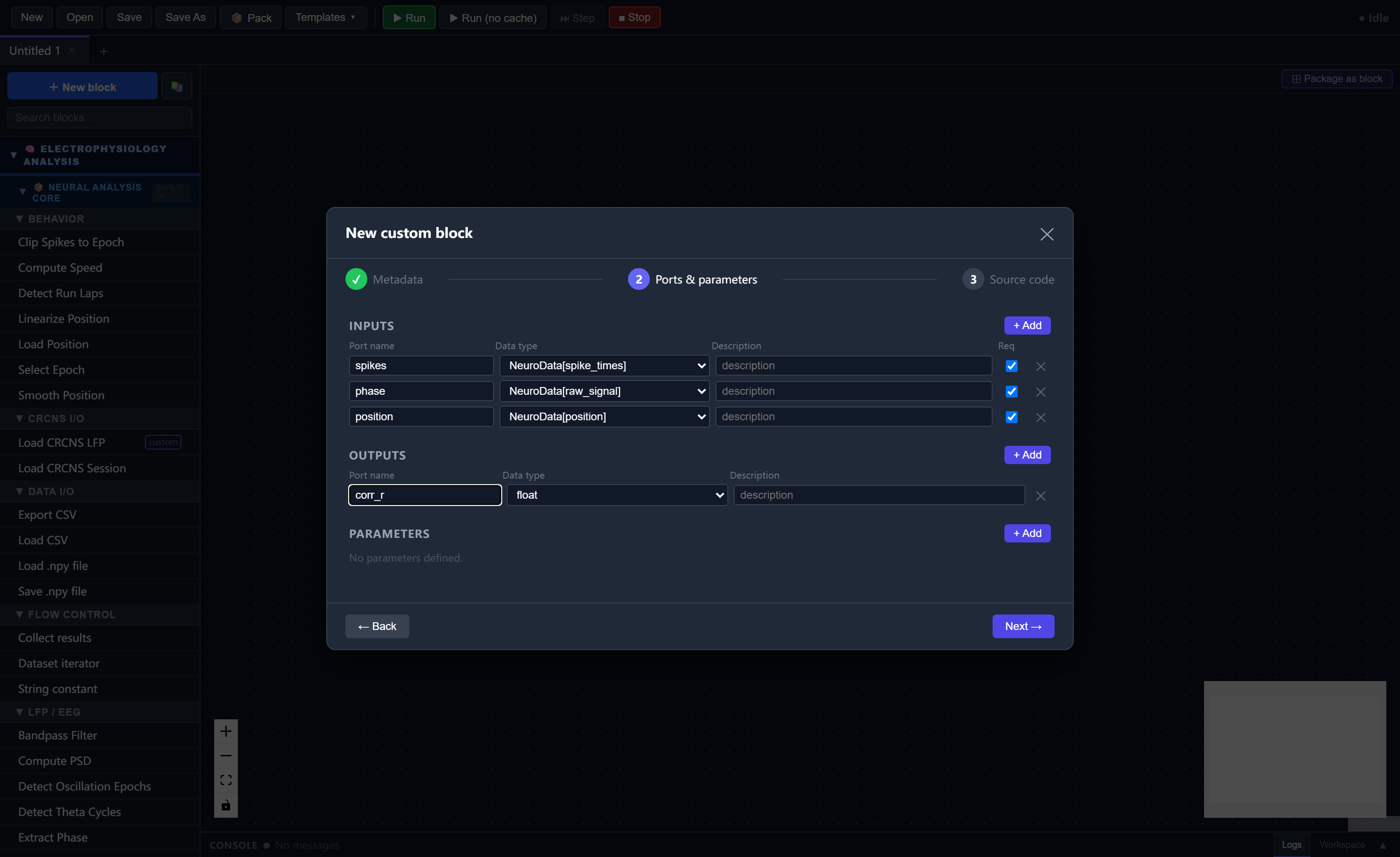
Click Next.

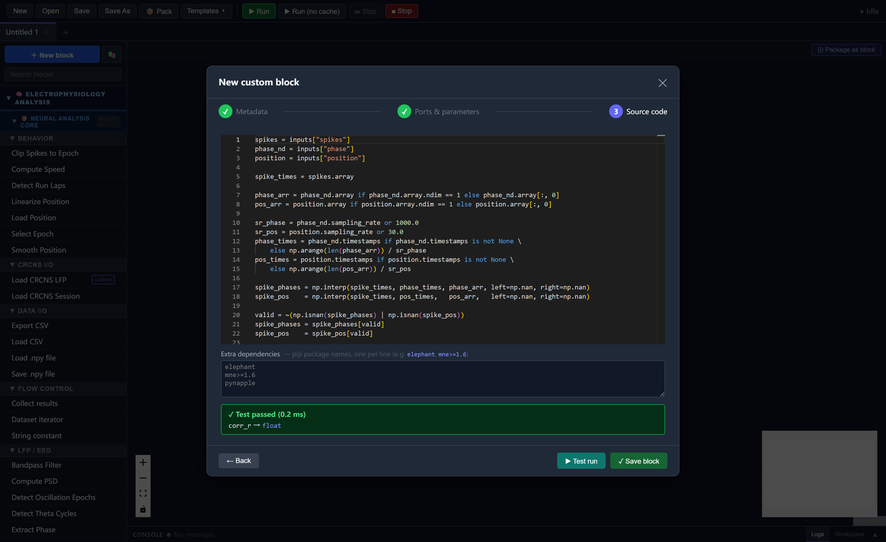
3.4 Step 3 — Source Code

Replace the template body with:

spikes = inputs["spikes"]
phase_nd = inputs["phase"]
position = inputs["position"]

spike_times = spikes.array

# Get phase and position arrays
phase_arr = phase_nd.array if phase_nd.array.ndim == 1 else phase_nd.array[:, 0]
pos_arr = position.array if position.array.ndim == 1 else position.array[:, 0]

# Build time axes
sr_phase = phase_nd.sampling_rate or 1000.0
sr_pos = position.sampling_rate or 30.0
phase_times = phase_nd.timestamps if phase_nd.timestamps is not None \
    else np.arange(len(phase_arr)) / sr_phase
pos_times = position.timestamps if position.timestamps is not None \
    else np.arange(len(pos_arr)) / sr_pos

# Interpolate phase and position at each spike time
spike_phases = np.interp(spike_times, phase_times, phase_arr,
                         left=np.nan, right=np.nan)
spike_pos    = np.interp(spike_times, pos_times,   pos_arr,
                         left=np.nan, right=np.nan)

# Drop spikes outside the recorded range
valid = ~(np.isnan(spike_phases) | np.isnan(spike_pos))
spike_phases = spike_phases[valid]
spike_pos    = spike_pos[valid]

# Pearson correlation — negative r means phase decreases as position increases
corr_r = float(np.corrcoef(spike_phases, spike_pos)[0, 1])
disp(f"Phase precession r = {corr_r:.4f}")

return {"corr_r": corr_r}

Built-in helpers

numpy is always available as np. disp() prints to the run progress console.

Click Test Run to verify the block works, then Save Block.

3.5 Connect the new block

Drag Get Phase Precession R from the side panel onto the canvas. Connect its inputs:

From block	Port	→	To port
extract_phase	phase	→	phase
load_spike_times	spikes	→	spikes
linearize_position	linear_pos	→	position

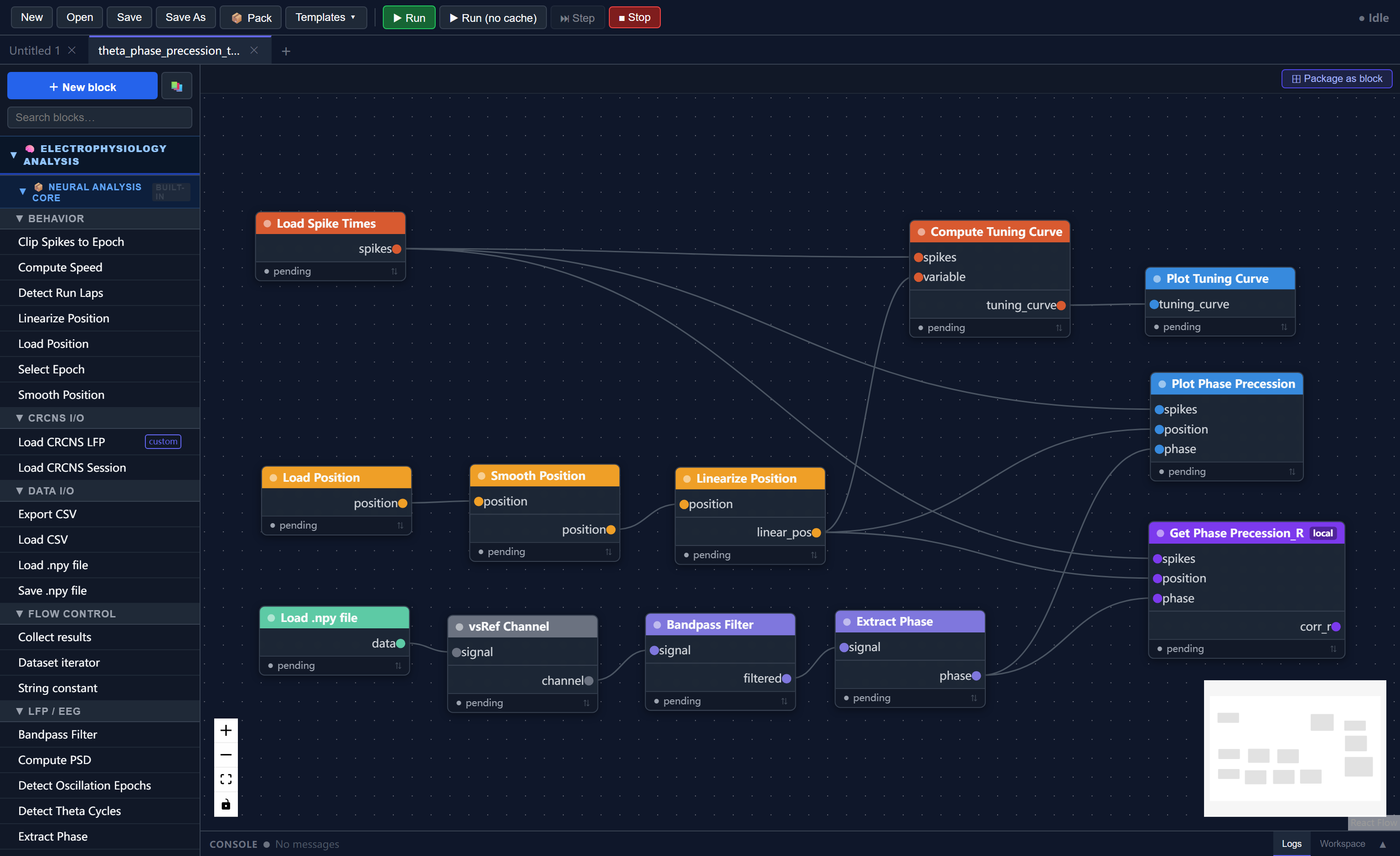
3.6 Save and run

Save as theta_phase_precession_test1.json. Click Run. The progress panel prints:

Phase precession r = -0.3821

A more negative value indicates stronger phase precession.

---

Part 4 — Composite Blocks and Multi-Session Analysis

You now have a complete working workflow. Here you will package it as a composite block — a single reusable node that encapsulates the entire pipeline — and use it to process two sessions in parallel.

4.1 Package the workflow as a composite block

With theta_phase_precession_test1.json open, click ⊞ Package as block in the canvas tab bar.

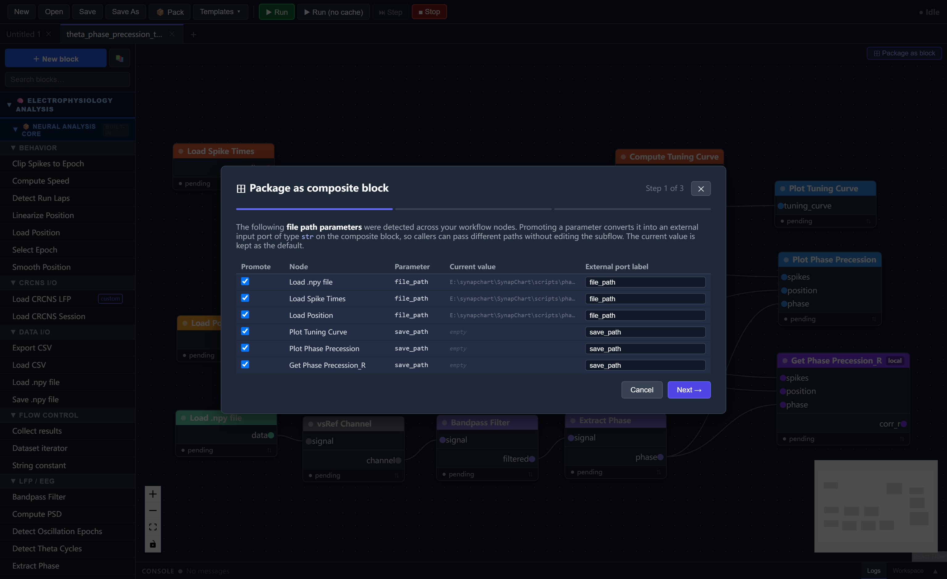
Step 1 — Promote file path inputs

Check all three file path parameters to expose them as input ports:

Promote	Node	Parameter	External port label
☑	Load LFP	file_path	lfp_path
☑	Load spike times	file_path	spike_path
☑	Load position	file_path	pos_path

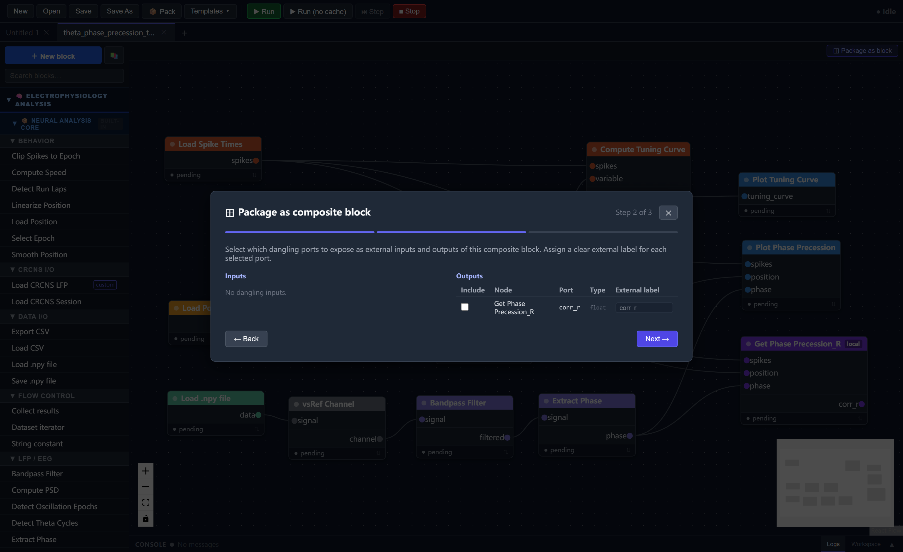
Step 2 — Select output ports

Check corr_r to expose it as an output:

Include	Node	Port	External label
☑	get_phase_precession_r	corr_r	corr_r

Step 3 — Metadata

Field	Value
Block name	PhasePrecession
block_type_id	phaseprecession
Category	Composite
Description	Full theta phase precession pipeline. Accepts three file paths and outputs the phase-position correlation coefficient.

Click Save composite block. The block appears in the side panel under Composite.

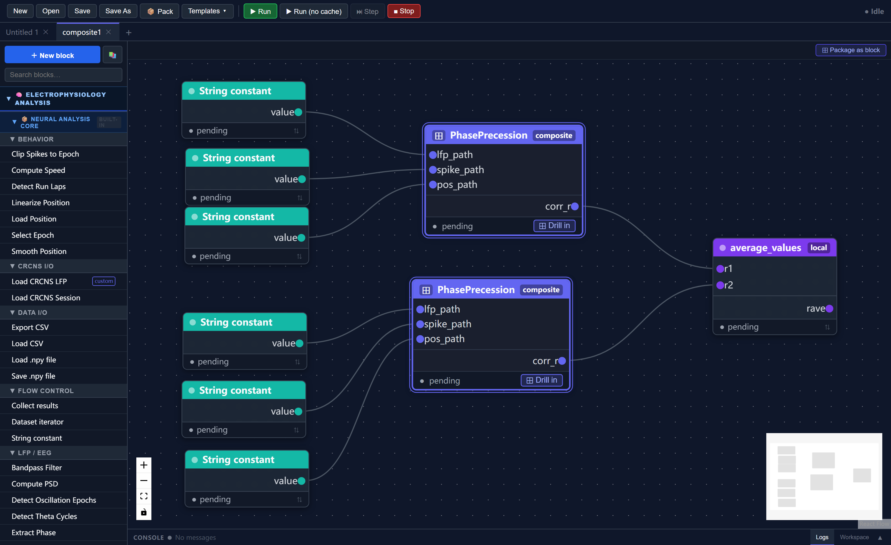
4.2 Build the multi-session workflow

Click New in the toolbar to start a fresh canvas.

Add two PhasePrecession composite blocks — drag PhasePrecession from the side panel twice.

Add six String constant blocks — find String constant under Flow control and add six. Set their value parameters:

Session 1:

Value
C:\path\to\backend\scripts\phase_precession_1_lfp.npy
C:\path\to\backend\scripts\phase_precession_1_spikes.npy
C:\path\to\backend\scripts\phase_precession_1_position.npy

Session 2:

Value
C:\path\to\backend\scripts\phase_precession_2_lfp.npy
C:\path\to\backend\scripts\phase_precession_2_spikes.npy
C:\path\to\backend\scripts\phase_precession_2_position.npy

Replace C:\path\to\backend\scripts\ with the actual path on your machine.

Connect the string constants to the matching ports on each composite block (lfp_path, spike_path, pos_path).

Add an average_values local block — click + New Block and create:

• Name: average_values
• Inputs: r1 (float), r2 (float)
• Output: rave (float)
• Source code:

r1 = float(inputs["r1"])
r2 = float(inputs["r2"])
rave = float((r1 + r2) / 2)
disp(f"averaged_corr_r = {rave:.4f}")
return {"rave": rave}

Connect both composite blocks' corr_r outputs to r1 and r2.

4.3 Save and run

Save as composite1.json. Click Run.

Both PhasePrecession blocks execute their full internal pipelines. The progress panel prints:

[PhasePrecession / session 1] Phase precession r = -0.3821
[PhasePrecession / session 2] Phase precession r = -0.4103
averaged_corr_r = -0.3962

Drilling into a composite block

Click the ⊞ Drill in button at the bottom of any composite node to inspect its internal workflow in a nested canvas tab. Double-click any internal block to edit its parameters without leaving the view.

---

Summary

In this tutorial you:

1. Ran a template theta phase precession workflow on synthetic hippocampal data
2. Created a custom get_phase_precession_r block quantifying precession strength as a Pearson correlation
3. Packaged the workflow as a PhasePrecession composite block with promoted file path inputs and a corr_r output
4. Built a two-session parallel analysis that averages the correlation across sessions

---

Next Steps

• Tutorial 2: Using the dataset iterator to batch-process all three sessions automatically with a CSV file
• Tutorial 3: Theta sequences with real hippocampal data — loading a CRCNS HC-11 session and analyzing direction-specific neural dynamics
• Block Reference — full documentation of all built-in blocks and their parameters