Getting Started
SynapChart is a visual pipeline builder for neuroscience data analysis. You wire together blocks — each wrapping a single analysis step — into a workflow, then run the whole pipeline with one click.
Installation
Requirements
- Windows, macOS, or Linux (SynapChart is pure Python + a browser UI; the CI test suite runs on Linux across Python 3.10–3.12)
- Python 3.10 or later (download)
- A virtual environment (
venvor conda) is recommended to keep the install isolated
Install
# Recommended: install into a clean virtual environment
python -m venv synapchart-env
# Windows:      synapchart-env\Scripts\activate
# macOS/Linux:  source synapchart-env/bin/activate

pip install synapchart
Prefer conda?
conda create -n synapchart python=3.11 && conda activate synapchart, then
pip install synapchart, works just as well.
Launch
synapchart
SynapChart starts a local server and opens your browser automatically at http://localhost:8000. Keep the terminal open while working — press Ctrl+C to stop the server when done.
Something not working?
- Browser didn't open? Go to
http://localhost:8000manually. - Port already in use? Start on another port:
synapchart --port 8123. synapchart: command not found? The environment where you ranpip installisn't active — re-activate it, or runpython -m backend.cli.
Your first pipeline (about 5 minutes)
The fastest way to see SynapChart produce a real result is to run a built-in template on the example data.
Templates ship with the package; the example data is generated
The example workflow templates are bundled with SynapChart, so the Templates menu is populated the moment you install. The tutorial datasets are not shipped — you generate them with a small script from the repository. The easiest way to get that script (and a working directory) is to clone the repo:
git clone https://github.com/yuchenz93/SynapChart.git
cd SynapChart
-
Generate the example data — three synthetic hippocampal sessions:
python scripts/generate_phase_precession_data.pyThis writes
phase_precession_1_lfp.npy,_spikes.npy,_position.npy(and_2_,_3_) into thescripts/folder. -
Launch SynapChart (from anywhere — templates are bundled):
synapchart -
In the toolbar click Templates → Tutorial → theta_phase_precession. A 10-block pipeline loads on the canvas.
-
Double-click each of the three Load blocks and set its
file_pathto the matching file from step 1 (…/scripts/phase_precession_1_lfp.npy, etc.). -
Click Run. Two plots appear — a place field and a theta phase-precession scatter. That's a complete analysis pipeline.
Tutorial 1 builds this same result step by step, then extends it with a custom block and a reusable composite block.
The Interface
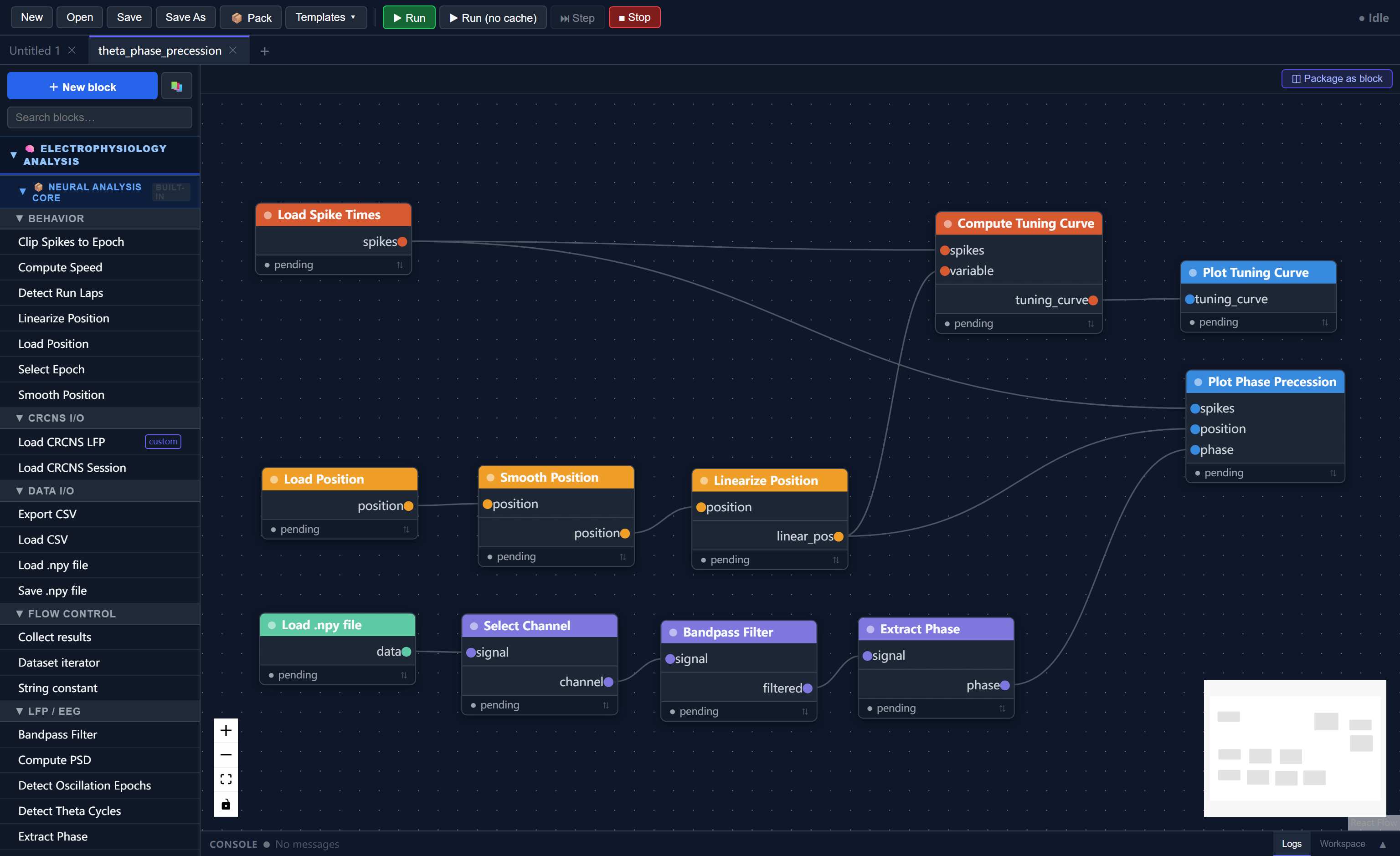
SynapChart has four main areas:
① Side Panel (left)
The block library. All available blocks are listed here, grouped by library and category. Use the search box at the top to filter by name or description. Drag any block from this panel onto the canvas to add it to your workflow.
The + New Block button opens the block creation wizard for writing a custom Python block.
② Canvas (center)
The main workspace. Each block appears as a node with input ports on its left edge and output ports on its right edge. Connect two blocks by clicking and dragging from an output port to an input port. Scroll to zoom, drag the background to pan.
Double-click any block to open its parameter editor.
③ Toolbar (top)
| Control | Action |
|---|---|
| New / Open / Save | File operations |
| Templates | Load a pre-built example workflow |
| Run | Execute the full pipeline |
| Stop | Cancel a running pipeline |
④ Run Progress Panel (bottom)
Appears while a pipeline is executing. Shows each block's status in execution order, a real-time progress bar, and any console output (disp() calls) printed by blocks.
The Block Library
The side panel organises blocks into libraries (blue headers) and categories (grey sub-headers).
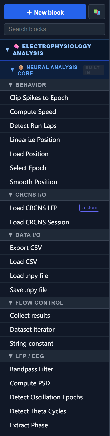
Built-in libraries
| Library | Contents |
|---|---|
| Neural Analysis Core | LFP/EEG, spikes, behavior, decoding, visualization, and data I/O primitives |
| 1D Maze Analysis | State-aware analysis for linear track experiments (tuning curves, phase precession, replay) |
| 2D Maze Graph Analysis | Graph-theory-based place map and replay analysis for open-field mazes |
These three libraries are grouped under the Electrophysiology Analysis section in the sidebar.
User Blocks
Your custom and composite blocks appear under User Blocks, separated by category. Blocks you create are stored permanently in backend/blocks/ and available across all workflows.
Searching
Type in the search box at the top of the side panel to filter blocks across all libraries simultaneously. The panel collapses to show only matching blocks.
Block Types
Standard blocks
A standard block runs a single Python function. It has typed input and output ports and optional parameters you set in the parameter editor. Most built-in blocks are standard blocks.
Custom blocks
Click + New Block to open the block wizard and write your own Python block. You define ports, parameters, and a run() function body. The wizard includes a live test runner and a Monaco code editor.
See Custom Blocks for a step-by-step guide.
Composite blocks
A composite block wraps an entire subflow into a single reusable node. Clicking ⊞ Package as block in the canvas tab bar opens the packaging wizard — it lets you promote internal parameters as input ports and expose output ports on the block's surface.
Click the ⊞ Drill in button at the bottom of any composite node to inspect its internal workflow in a nested canvas tab.
See Composite Blocks for details.
Workflows
Templates
Click Templates in the toolbar to browse pre-built workflows organised by category. Selecting a template opens it in a new tab with all blocks and connections already in place. Templates are a good starting point — modify them freely without affecting the original.
Saving and loading
Use Save to write the current canvas to a .json file. The file is self-contained: it embeds any custom or composite block definitions used in the workflow, so collaborators can open it without having those blocks installed.
Smart caching
On the first run all blocks execute from scratch. On subsequent runs, SynapChart detects which blocks have unchanged inputs and parameters and skips them, loading their outputs from cache instead. Only the modified branches re-execute. This makes iterative development fast even on large datasets.
Next Steps
- Tutorial 1: Theta Phase Precession — build a complete analysis pipeline from scratch using synthetic hippocampal data
- Block Reference — full documentation of all built-in blocks
- Custom Blocks — write and register your own analysis steps
- Composite Blocks — package workflows as reusable blocks